1.4.2. Matrix and interaction network.
This method is used for determination of relations between elements within the investigated problem. To build interaction matrix, firstly, it is necessary to determine notions of "element" and "interrelationship". Then, each element is compared with another one, and probable existence of interrelations between each group of elements is determined on the basis of these datum.
Let's consider this method on a simple model example.Figure.l.8,a. demonstrates a design, of crankpin joints.
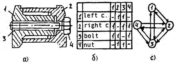
Fig 1.8. Matrix and interaction network of initial design of a "crankpin" assembly unit:
1 - left crankpin; 2 - right crankpin; 3- bolt; 4 - nut
Details here are considered to be elements and their joint-interaction. If the details are connected with each other directly, such interaction is specified by index 1, if no-0. Interaction matrix of this assembly unit is showed at fig.l.S.b.
Using this figure, first of all it is possible to determine the most loaded details (maximum number of interactions). Such information is especially important, if an assembly unit is a complex one, as it is practically impossible to carry out such evaluation only with the help of intellectual means, without using supporting ones. Then on basis of received information it is possible to take some decisions. For example, on design modernization or simplification.
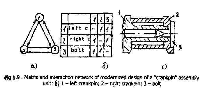
If we want to show interaction matrix graphically, it is possible to present elements in the form of circles, and interaction between them as lines with arrows, pointing to the direction of interaction. Then, we'll receive a scheme, called "interaction network", fig.l.S.c. It permits to visualize the investigated object's structure. It is seen, that interrelations between details 1-3 and 2-4 are crossed, thus the topological structure of this network is unsuccessful. It can be simplified in some ways.Fig.l.9.a. demonstrates one of simplification variants of interaction network. The interaction matrix is described on the basis of new structure (fig.l.9.b), and fig.i.9.c. demonstrates new simplified construction decision on the same crankpin.
Íŕçŕä Îăëŕâëĺíčĺ Âďĺđĺä